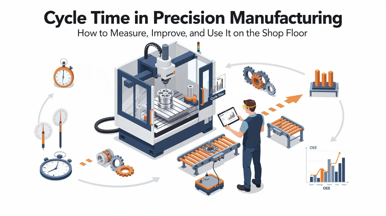
Cycle Time in Precision Manufacturing: How to Measure, Improve, and Use It on the Shop Floor

Every second on the shop floor carries a cost. Whether you run a CNC cell, a die casting line, or a sheet metal fabrication bay, understanding cycle time is the starting point for controlling that cost. This guide walks through what cycle time actually means in precision manufacturing, how to calculate cycle time, where losses hide, and what you can do about them. If you source custom parts from an OEM supplier, the information here will help you ask better questions and evaluate manufacturing partners more critically.

What is cycle time in manufacturing?

Cycle time measures the time to complete one unit at a specific operation in a manufacturing process. In discrete precision manufacturing-CNC machining, die casting, sheet metal fabrication-it refers to the elapsed time from the moment work begins on a part until that operation is considered complete. For a CNC milling step on an aluminum housing, cycle time runs from first tool engagement to final cut. For a die casting shot, it covers injection through ejection.

In shop-floor practice, cycle time typically includes active processing time plus minor in-cycle waits (tool changes within the program, spindle repositioning) but excludes long downtimes, transport between workstations, or setup delays that belong to separate tracking categories.

There is a practical distinction between per-piece and per-batch cycle times. Consider machining 50 stainless-steel shafts on a turning center: if 240 minutes of net production time yields 48 good pieces, the per-piece cycle time is 5 minutes. In die casting, a multi-cavity mold might produce 20 parts per 30-second shot, giving an effective per-piece time of 1.5 seconds.

Understanding actual cycle times is essential for accurate quoting-especially when tolerances reach ±0.002 mm-for capacity planning, and for keeping on-time delivery commitments to overseas OEM customers who depend on predictable schedules.

Cycle time vs. lead time vs. takt time

Cycle time is often confused with lead time and takt time. All three are key metrics, but they answer different questions.

Metric	What it measures	Example
Cycle time	Time to process one unit at one process step, from the moment work begins to completion	5-axis milling a titanium implant bracket: 6 minutes
Lead time	Total elapsed time from customer order to delivery, including queue time, procurement, all operations, finishing, inspection, packing, logistics	Same bracket: 18 days order-to-delivery
Takt time	Required production pace to meet customer demand: available production time ÷ required units	40 hours/week ÷ 1,000 units = 2.4 minutes/unit

The difference between cycle time vs lead time is significant. A machined aluminum enclosure might have a 6-minute machining cycle time, but its lead time stretches to 18 days once you account for raw materials sourcing, anodizing, inspection, and international shipping. From the customer’s perspective, lead time includes order processing and delivery time-every day matters.

The gap between cycle time vs takt time reveals capacity risk. Takt time indicates the pace needed to meet customer demand. If an automotive OEM needs 600 parts per week and available machining time is 40 hours, takt time is 4 minutes per unit. But if the bottleneck CNC machine runs at 5 minutes per unit, if cycle time exceeds takt time, production cannot meet demand without adding machines, shifts, or process improvements.

Aligning cycle time and lead time with takt time is a core principle of lean manufacturing and continuous improvement.

Types of cycle time and related manufacturing terms

Several variants help clarify exactly what you are measuring on the shop floor.

Ideal cycle time is the theoretical minimum achievable under perfect conditions-based on machine specifications, CAM simulation, or best-observed runs. It represents the benchmark against which actual performance is compared.

Actual cycle time is the real measured time spent per part, including minor slowdowns, in-program pauses, tool wear compensation, and operator-imposed adjustments. This is the actual time spent working on each piece.

Effective machine cycle time rolls in load/unload and changeover overhead divided by batch size. Effective cycle time includes active production time plus setup and waiting, making it useful for CNC and die casting cells where material handling is a constant factor.

Processing time vs. non-value-creating time: processing time covers value added time-cutting, forming, finishing. Non value added time includes waiting time for an available CMM, searching for fixtures, manual deburring, or rework after a failed inspection. Separating these reveals where idle time inflates the total.

Production lead time and throughput time span the full manufacturing process from raw material receipt to shipment. Cycle time can vary significantly across different industries and even across operations within the same facility-turning might take 3 minutes, while anodizing takes 45 minutes per batch.

At Anebon, we track both operation-level cycle times (turning, milling, anodizing) and order-level lead times to manage throughput and meet customer commitments across aerospace, automotive, and medical device programs.

How to calculate cycle time on the shop floor

The standard cycle time formula is straightforward:

Cycle Time = Net Production Time ÷ Total Units Produced

Net production time excludes breaks and downtime in cycle time calculation. It includes run time plus minor, acceptable in-cycle pauses but strips out major equipment failures, shift breaks, and material delays. Cycle time is calculated as total production time divided by units produced-consistency in what you include determines whether the number is useful.

CNC machining example: A shift yields 240 minutes of net machining time and 48 good aluminum brackets. Average cycle time = 240 ÷ 48 = 5.0 minutes per bracket. For a deeper look at the math behind turning operations, see our guide on how to calculate CNC turning cycle time.

Die casting batch example: A cold-chamber aluminum process runs a 30-minute cycle to cast and trim a batch of 20 parts. Batch cycle time is 30 minutes; effective per-piece time is 1.5 minutes.

Multi-step sheet metal example: A laser-cut electronics chassis moves through laser cutting (45 seconds), bending (30 seconds), welding (60 seconds), and powder coating (120 seconds). Total critical-path cycle time is 255 seconds, roughly 4.25 minutes per unit.

Consistent start/stop definitions matter. Whether you measure clamp-to-unclamp or first-cut-to-last-cut, keeping it the same over months makes data comparable. Use time studies, machine counters, and ERP system data logging rather than rough estimates-especially for tight-tolerance work where setup and inspection influence the real numbers. Cycle time helps optimize production planning and scheduling when the data behind it is trustworthy. For more on estimating machining durations, see how to estimate CNC machining time.

Cycle time, lead time, and customer satisfaction

Shorter cycle times improve customer satisfaction and competitiveness. When cycle times are stable and predictable, lead time promises hold up, and OEM assembly lines stay on schedule. When they are not, the ripple effects-missed shipments, expedited freight costs, production line stoppages-damage relationships and raise operational costs.

Cycle time impacts operational costs and profitability directly. Increased cycle times often reduce profits and efficiency in manufacturing because machine-hour rates keep accumulating while fewer parts come off the line. Conversely, decreasing cycle time allows production of more goods within the same timeframe, improving cost per part without additional capital investment.

The connection between cycle time and lead time is not abstract. Consider a realistic scenario: by reducing cycle times through dynamic feed rate adjustments, Anebon cut the turning cycle time on a stainless-steel shaft by 15%-from 10 to 8.5 minutes per part. That improvement, compounded across hundreds of units, trimmed order lead time from 20 to 16 days for a European robotics OEM, enabling faster delivery without sacrificing quality.

These gains are not limited to manufacturing. Accenture reduced request-to-order cycle time by 50%, enhancing customer experience across its operational processes. Tech Data cut procure-to-pay cycle time by 57%, ensuring customer satisfaction through faster order fulfillment. The principle holds everywhere: speed and consistency build trust.

In precision metal fabrication, however, faster cycle time must never compromise quality. Scrap and rework erase time gains immediately, so any process improvement initiatives must preserve tolerances, surface finish, and dimensional accuracy.

Cycle time loss and identifying bottlenecks

Cycle time loss occurs when production runs slower than ideal. The gap between what a machine or process should achieve and what it actually delivers, multiplied across volume, represents hidden waste that accumulates daily.

The formula is simple:

Cycle Time Loss = Actual Run Time − (Total Units × Ideal Cycle Time)

If ideal cycle time for turning a part is 3 minutes and you produce 1,000 units, ideal run time is 3,000 minutes. If actual run time is 4,000 minutes, you have 1,000 minutes of cycle time loss-over 16 hours of waste in a single run. Cycle time loss increases operational costs and reduces efficiency across the entire value stream.

Cycle time is crucial for identifying bottlenecks in processes. Typical causes of loss in precision manufacturing include:

• Suboptimal feeds and speeds (conservative programming to protect tools)

• Frequent tool changes and worn cutting tools

• Small unplanned stops for chip evacuation or thermal stabilization

• Manual deburring or cleaning between operations

• Searching for fixtures, gauges, or unnecessary steps in the workflow

Cycle time is heavily influenced by workflow bottlenecks, equipment maintenance, and human variability. Bottlenecks occur when a specific machine operates slower than others, creating queues that stall production moving downstream. Tracking cycle times at workstations helps identify production bottlenecks-the longest, most heavily loaded operation (often 5-axis milling or CMM inspection) typically dictates overall throughput.

Practical tools for identifying bottlenecks include value stream mapping, line balancing, and Pareto charts of operation times. Cycle time is crucial for identifying operational issues before they compound into delivery failures. At Anebon, we routinely study bottleneck machines-high-precision grinders, CMMs, finishing stations-to improve overall flow rather than optimizing only low-impact steps.

Strategies to reduce cycle times in precision machining and fabrication

Optimizing cycle time requires targeted action on the operations that matter most. Here are proven strategies specific to CNC machining, die casting, and sheet metal fabrication:

Optimize cutting parameters. Adjusting feeds, speeds, and depth of cut using advanced tooling and process parameter optimization can materially reduce machining cycle times. High-efficiency milling (HEM) and adaptive clearing toolpaths push material removal rates higher without sacrificing surface finish. Enztec, a medical instrument manufacturer, used force-based optimization to reduce CNC cycle times by 16%, unlocking over 1,800 hours of machining capacity annually.

Apply SMED principles. For small-batch OEM work, reducing setup and changeover times with modular fixtures has outsized impact. Moving from 30-minute changeovers to under 10 minutes keeps production moving between product variants.

Reorganize workstations with 5S. Minimize walking, searching, and handling around CNC cells and bending stations. Eliminating unnecessary steps in material staging alone can save minutes per shift.

Automate repetitive tasks. Pallet changers, bar feeders, robotic loading, and in-machine probing reduce manual touches and idle time. Osvald Jensen, a gear manufacturer, cut cycle time by 44% by upgrading automation in machine tending with a dual-gripper robot-without changing machining parameters.

Combine operations. Using 5-axis machining instead of multiple setups eliminates repositioning and reduces total cycle time while improving accuracy through one process flow.

Pursue continuous improvement. Businesses minimize cycle time by automating tasks and standardizing procedures. Regularly review measured cycle times, test incremental changes, and standardize best methods across shifts through feedback loops. Credibom improved overall cycle time by 5% to 10% through systematic process optimization. Process mining can reduce cycle time significantly when applied to identify opportunities hiding in production data.

Cycle time in lean manufacturing and continuous improvement

Lean manufacturing principles focus on reducing waste-waiting, motion, over-processing, defects-that inflates cycle times without adding real value. Every second of non-value-creating activity is a target for elimination.

Comparing cycle time to takt time drives capacity decisions. When a critical operation cannot meet demand at current cycle times, lean thinking prescribes specific responses: rebalance work across stations, change methods, or add enough capacity to close the gap. The goal is to streamline processes so that one unit flows through without unnecessary delays.

Kanban and pull systems rely on stable cycle times to correctly size containers and limit work-in-progress. When cycle times fluctuate, WIP builds up unpredictably, inventory costs rise, and the pull system breaks down.

Cycle time analysis also feeds into OEE (Overall Equipment Effectiveness) by exposing slow cycles and small stops on critical machines. The Performance component of OEE uses the ratio of ideal to actual cycle time-errors in defining either lead to misleading metrics and misdirected effort.

At Anebon, ISO 9001:2015 and ISO 14001:2015 frameworks provide the structure for standard process documentation, statistical analysis of performance data, and continuous improvement projects focused on cycle time and quality. Shorter cycles often mean lower electricity and coolant consumption, supporting both cost and environmental goals-operational excellence with a smaller footprint.

Practical examples: cycle time in CNC machining, die casting, and sheet metal

Example 1: CNC Machining – Aerospace Aluminum Bracket

A 5-axis machining cycle for an aerospace bracket originally ran at 12 minutes per part across multiple setups. After machining parameter trade-off analysis-including toolpath optimization, cutter selection, and single-setup fixturing-cycle time dropped to 9.5 minutes. Over a 2,000-piece order, this saved 83 machine-hours, cutting lead time by 4 days and allowing the team to accept a rush order from an automotive OEM that same month.

Example 2: Die Casting – Zinc Components

A zinc hot-chamber die casting process for small connector housings originally cycled at 45 seconds per shot. Improved cooling channel design and automated trimming reduced cycle time to 35 seconds-a 22% improvement that increased hourly throughput from 80 to 103 shots. This gave the production team a competitive edge on high-volume electronics orders while keeping scrap below 1%.

Example 3: Sheet Metal – Electronics Chassis

A laser cutting and bending process for an electronics chassis had a combined cycle time of roughly 4.3 minutes per unit. Nesting optimization in the laser step, offline bend programming, and better material staging cut total cycle time by 20% to about 3.4 minutes per chassis. The savings translated directly into lower cost per part and enough buffer to handle 15% demand surges without overtime-a clear benefit from the customer’s perspective.

Measuring and tracking cycle time with digital tools

Accurate time tracking is foundational. Machine controllers, sensors, and counters can log start/stop events for each cycle-spindle-on/spindle-off, clamp/unclamp-providing granular data without manual effort.

ERP/MES systems store standard (planned) cycle times and compare them with actual performance captured from the shop floor. This comparison highlights variances in real time, turning raw data into actionable analysis capabilities. When actual time drifts above standard by a set threshold (say 10%), alerts trigger engineering review before quality suffers.

For operations not yet fully digitized-manual assembly, deburring, packaging-simple time studies with observation remain effective. Recording not just averages but distributions (min, max, standard deviation) reveals instability that undermines scheduling even when the average looks acceptable.

Accurate cycle time data is necessary for reliable CNC machining cost calculation, quoting, and production scheduling, especially when serving multiple industries simultaneously. At Anebon, we use a combination of digital data capture and on-site engineering reviews to keep standard cycle times realistic and to identify opportunities for process optimization across our CNC, die casting, and sheet metal operations.

How Anebon uses cycle time to support OEM customers

At Anebon, process efficiency starts before the first chip is cut. From the DFM (design for manufacturability) stage, our engineers select fixtures, tooling, and operational sequences with cycle time in mind-recommending uniform wall thickness in die cast parts to reduce cooling time, or combined setups in machining to eliminate repositioning.

Early prototype runs measure real cycle times under production-realistic conditions. This data refines quotations and lead time commitments before full-scale production begins-no surprises mid-run.

Stable, optimized cycle times let us offer competitive pricing, reliable delivery windows, and consistent quality across CNC machined, die cast, and sheet metal parts. Overseas OEMs benefit from reduced risk of delays, clearer schedules, and the ability to ramp volumes up or down based on shifting customer demand.

While cycle time concepts also appear in project management, software development, and agile teams, the stakes in precision manufacturing are physical: every minute saved on the shop floor compounds into lower operational costs, better process efficiency, and a stronger customer experience.

Ready to optimize processes for your next production run? Share your drawings with Anebon’s engineering team. We will evaluate cycle times, identify bottlenecks, and propose a manufacturing plan that meets your cost, quality, and delivery targets. Request a quote today.